Introduction
Revenue management has become a critical function for airlines, with dynamic pricing algorithms adjusting fares in real time based on demand forecasts, inventory levels, and competitive conditions. Despite decades of practice, many airlines still rely on heuristic rules that may deviate substantially from optimal pricing policies.
In this paper, we develop and estimate a structural model of dynamic pricing that allows us to recover the airline's underlying demand parameters and compute optimal booking limits and price paths. We apply the model to proprietary booking data from a major European carrier operating on short-haul routes, covering approximately 2.3 million booking observations across 180 days before departure.
Model
Consumer Demand
We model consumer demand using a discrete-choice framework. In each period $t$, a random number of potential travelers arrive and choose among available fare classes or an outside option. The utility of consumer $i$ for fare class $j$ is:
where $p_{jt}$ is the fare, $\tau$ is a threshold number of days before departure capturing business vs. leisure segmentation, and $x_{jt}$ includes flight characteristics. The error term $\varepsilon_{ijt}$ is i.i.d. Type I extreme value.
Firm's Optimization Problem
The airline chooses prices for each fare class to maximize expected revenue subject to capacity constraints. Let $C$ denote total seat capacity and $Q_{jt}(p_t)$ the expected demand for class $j$ given the vector of prices $p_t$. The airline's problem in period $t$ with remaining capacity $c$ is:
The first term represents current-period revenue, while the second captures the continuation value of remaining inventory. The expectation is over the random demand realization $q_{jt}$.
Dynamic Programming Solution
We solve the dynamic program via backward induction. The terminal condition is $V_T(c) = 0$ for all $c$, since unsold seats have no salvage value. The first-order condition for the optimal price in each period balances the marginal revenue from a higher price against the marginal cost of reduced demand, which includes both the lost immediate revenue and the shadow value of capacity:
Data
Our dataset comprises booking records from a major European airline operating on 45 short-haul routes (under 1,500 km) between January 2023 and December 2024. Each observation includes the booking date, departure date, fare class, channel (direct website vs. OTA vs. corporate), and customer segment inferred from booking patterns.
| Variable | Mean | Median | Std.Dev. |
|---|---|---|---|
| Fare (€) | 142 | 118 | 87 |
| Days before departure | 47 | 35 | 38 |
| Booking lead time (days) | 42 | 31 | 36 |
| Load factor (%) | 84.2 | 86.0 | 11.3 |
Table 1: Summary Statistics (n = 2,341,000 booking observations)
Results
Elasticity Estimates
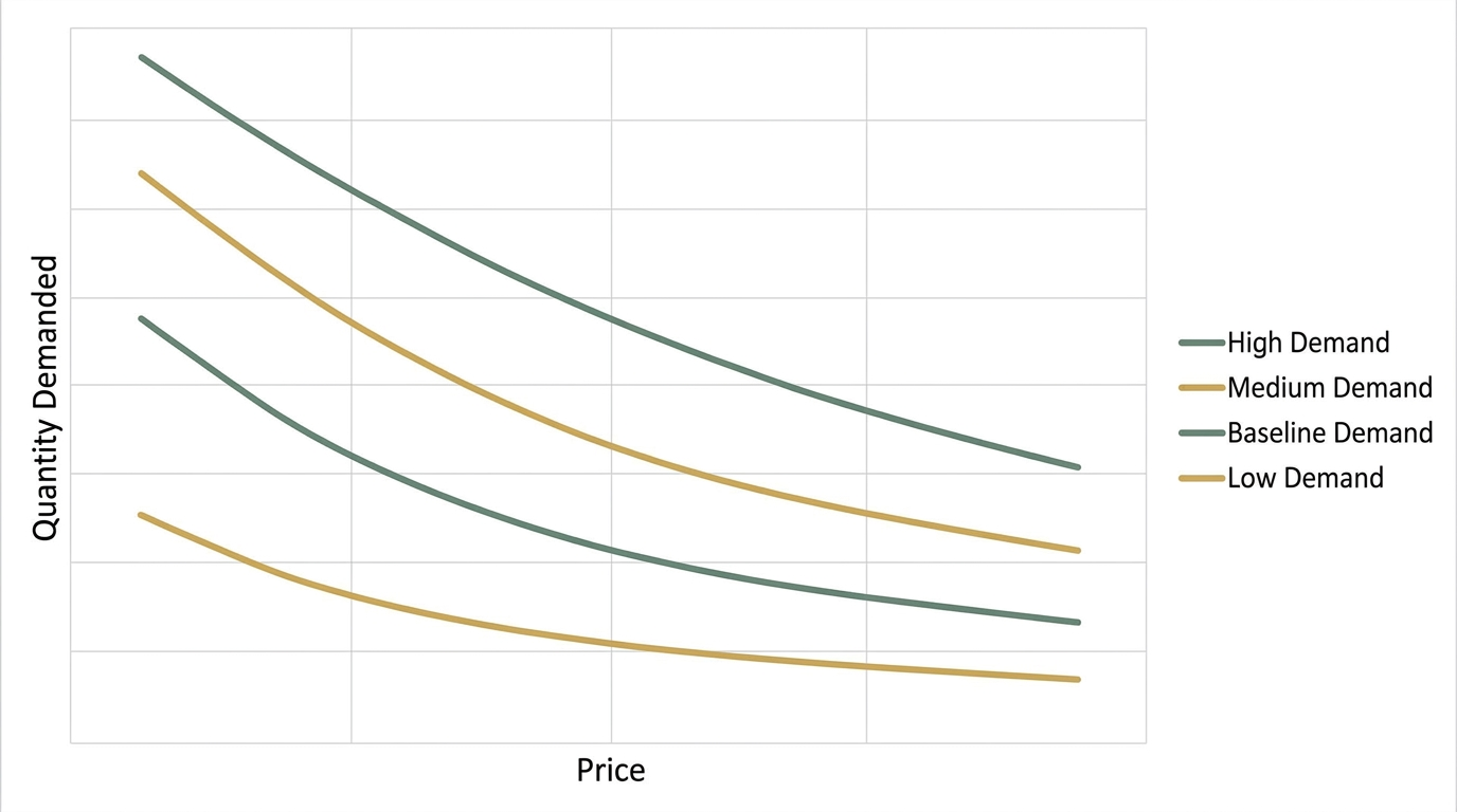
The estimated price elasticities vary substantially across customer segments and booking channels. Leisure travelers booking through OTAs exhibit the highest elasticity at −3.42, while corporate travelers booking direct show a much lower elasticity of −1.15. The time-to-departure effect is also strong: elasticities decrease (in absolute value) as departure approaches, reflecting the higher willingness-to-pay of last-minute bookers.
Optimal Policy
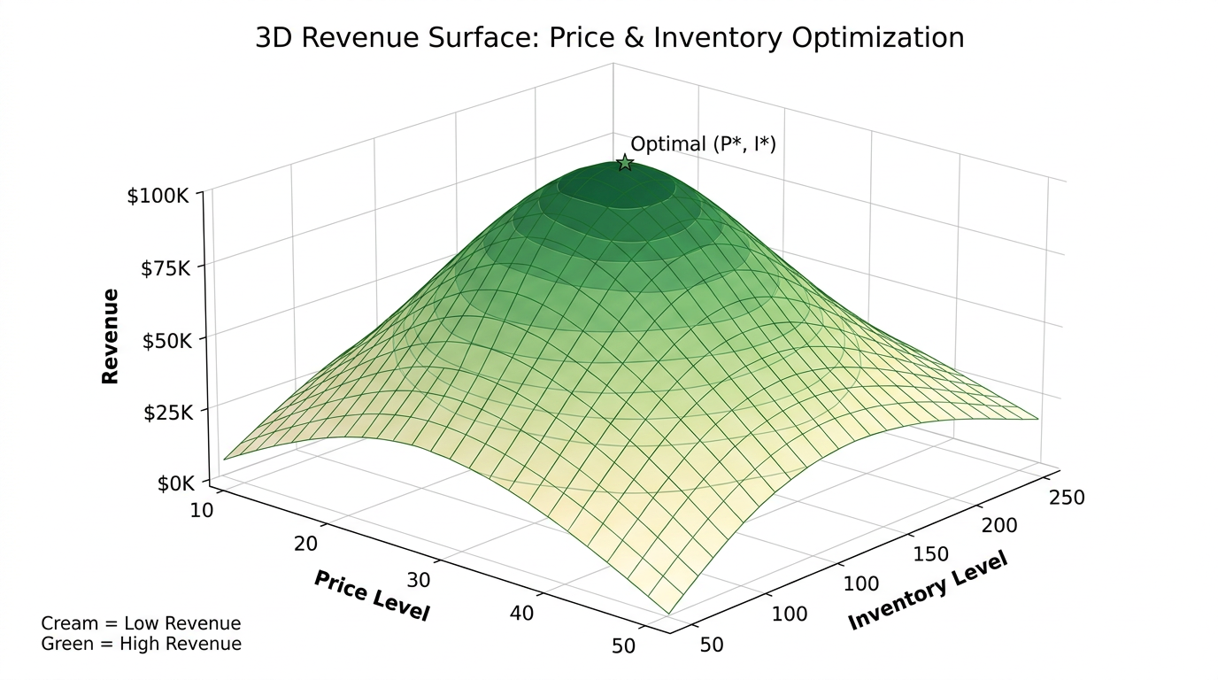
The optimal pricing policy exhibits significant inter-temporal price discrimination. Under the optimal policy, prices increase more steeply as departure approaches compared to the observed pricing. The airline should also close lower fare classes earlier than it currently does, reserving more capacity for higher-yield bookings.
Revenue Gains
We compare expected revenue under the optimal policy to observed revenue. The model predicts potential revenue gains of 4.7% on average across routes, with considerable heterogeneity. Routes with higher demand uncertainty and more dispersed willingness-to-pay show larger potential gains (up to 8.2%), while competitive trunk routes show smaller gains (around 2.1%).
Conclusion
This paper has developed and applied a structural model of dynamic pricing to airline revenue management. Our framework allows us to estimate demand parameters, compute optimal pricing policies, and quantify the revenue gains from improved pricing. The estimated potential gains of 4.7% represent a significant opportunity for the airline industry.
The model can be extended in several directions. First, incorporating competitor responses would allow for strategic pricing analysis. Second, adding no-show and overbooking decisions would provide a more complete revenue management framework. Third, applying the model to other industries with perishable inventory (hotels, car rentals) could yield additional insights.
References
- McFadden, D. (1978). “Modelling the Choice of Residential Location.” Transportation Research Record, 673, 72–77.
- Littlewood, K. (1972). “Forecasting and Control of Passenger Bookings.” AGIFORS Symposium Proceedings, 12, 95–117.
- Talluri, K. T., & van Ryzin, G. J. (2004). The Theory and Practice of Revenue Management. Springer.
- Escobari, D. (2012). “Dynamic Pricing, Advance Sales, and Price Discrimination.” Journal of Industrial Economics, 60(2), 274–298.
- Alderighi, M., Gaggero, A. A., & Piga, C. A. (2015). “Airline Scheduling and Pricing.” Journal of Transport Economics and Policy, 49(1), 95–114.